Image 1 of 1: ‘A visual representation of the above process showing the rule definitions, with arrows added to indicate the order wildcards and placeholders are substituted. Blue arrows start from the input of the `plot_avg_plaquette` rule, which are the files `intermediary_data/beta1.8/pg.plaquette.json.gz`, `intermediary_data/beta2.0/pg.plaquette.json.gz`, and `intermediary_data/beta2.2/pg.plaquette.json.gz`, then point down from components of the filename to wildcards in the output of the `avg_plaquette` rule. Orange arrows then track back up through the shell parts of both rules, where the placeholders are, and finally back to the target output filename at the top.’
Image 1 of 1: ‘Diagram showing jobs as coloured boxes joined by arrows representing data flow. A box labelled `avg_plaquette` is in red at the top left, and one labeled `ps_mass` is in green at the top right. From these, arrows lead into a yellow box labeled `one_loop_matching`. Incoming arrows into the top two boxes indicate the filenames `raw_data/beta2.0/out_pg` and `out_hmc` respectively. From the bottom an arrow points to the output filename, `intermediary_data/beta2.0/pg.corr.ps_decay_const.json.gz` ’
Figure 2
Image 1 of 1: ‘A DAG for the partial workflow with eleven similar columns, one per ensemble, each having a green `ps_mass`, a red `avg_plaquette`, and a yellow `one_loop_matching` job; each green and yellow box has an arrow leading to a green "spectrum" box at the bottom. ’
Image 1 of 1: ‘Representation of a computer with four microchip icons indicating four available cores. To the right are five small green boxes representing Snakemake jobs and labelled as wanting 1, 1, 1, 2 and 8 threads respectively. ’
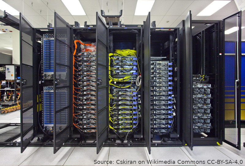
Image 1 of 1: ‘A photo of some high performance computer hardware racked in five cabinets in a server room. Each cabinet is about 2.2 metres high and 0.8m wide. The doors of the cabinets are open to show the systems inside. Orange and yellow cabling is prominent, connecting ports within the second and third racks. ’
Image 1 of 1: ‘Diagram showing three boxes in a row, connected from left to right by arrows. The boxes are labeled "`input_file`", "`data_file`", and "`output_file`". The arrows are labelled "`generate`" (24 hours), and "`plot`" (15 seconds). ’