Reproducible software environments

Overview

Teaching: 20 min
Exercises: 20 min

Questions

• Why do I need to document the software environment?

• How do I document what packages and versions are needed to reproduce my work?

Objectives

• Understand the difficulties of reproducing an undocumented environment.

• Be able to create a requirements.txt and environment.yml file.

So far, we have focused on getting the code that we have written in to a form where another researcher can run it in the same way. Unfortunately, this isn’t enough to ensure that the analysis we have done is reproducible. Each of the libraries we rely on in our code is constantly being developed and updated, as is the Python language, and the operating system that it runs on. As this happens, the default version to be installed on request will change. While minor version changes typically do not introduce any incompatibilities, eventually almost all software needs to introduce changes that break backwards compatibility in some way in order to develop and improve functionality available to new code. In the best case this will cause cosmetic changes, and the next best the code will fail to work at all because some function has been renamed, relocated, or removed. The worst case is when the code still runs without error, but gives a very different answer to that obtained with the old version of the library.

To make our analysis fully reproducible, we need to reproduce the entire computational environment that was used to perform it. In principle, this includes not only the version of Python and the packages that were installed, but also the operating system and the underlying hardware! For now, we will focus on reproducing as much of the original environment as we can.

Exporting environments with Conda

The Conda package manager used by Anaconda gives a way of exporting the current environment. This includes more than just Python packages; it also includes the specific Python version, as well as some dependency packages that would otherwise need to be installed separately. We can export our Conda environment as:

$ conda env export -f environment.yml
$ cat environment.yml

By convention the filename for conda environments is environment.yml; this file is in YAML format. Looking at it, we see it encodes the environment name, the Conda and Pip packages that we have installed, as well as the path to the environment on our computer.

If you don’t use Conda

We have used Conda here because it can define things quite precisely, including the version of Python and many external dependencies in addition to the Python packages being used. However, if you don’t use Conda, you can still export an environment.

The most basic way is built into Pip. Using pip freeze will output a list of all currently installed Pip packages. While this will not work if you are using Conda, since these packages are not available through PyPI, if all your packages were instead installed through Pip, then this gives a very commonly-accepted way to document your environment. By convention the filename for your list of packages is requirements.txt.

$ pip freeze > requirements.txt

Another alternative tool is called Poetry. This combines some of the functionality of pip freeze with some of the dependency and environment management aspects of Conda.

Trimming down an environment

We can see that this file is rather long; this is because we have exported the Anaconda base environment. This comes with a huge array of packages that could be useful for doing scientific computation. However, it means that it will be a lot of data to download for anyone who wants to recreate the environment, and a lot of that data will not be needed as it is packages we haven’t used. Instead, let’s create a new, clean environment to export, starting from Python 3.9

$ conda create -n zipf python=3.9
$ conda activate zipf

Now, we can install into this environment only the packages that we refer to in our Zipf code. If we haven’t documented all the requirements in the README yet, we can work out what these are by looking for any import statements in our code, and identifying those that are not either provided by our own code or by the Python standard library.

$ grep -r --no-filename import bin | sort | uniq

from collections import Counter
import argparse
import csv
import matplotlib.pyplot as plt
import pandas as pd
import string
import sys
import utilities as util

Of these, collections, argparse, csv, string, and sys are all part of the Python standard library, and utilities is part of our own code. That leaves Matplotlib and Pandas. Let’s install these with Conda:

$ conda install pandas matplotlib

If we’re using any tools installed without importing them, then they won’t be picked up by grep; in that case we need to check through our shell scripts to see if any commands are being run that need to be installed. If your analysis includes Jupyter Notebooks, for example, then you will need jupyter installed, even if you don’t ever use import jupyter.

Conda can also provide tools that aren’t Python packages, like curl. If you’re using a tool, or a specific version of a tool, that is likely to not be installed on everyone’s computer, then you should specify that too. curl is installed on most operating systems as of 2023, but it is possible that somsone will need it.

$ conda install curl

It’s a good idea to do a quick check now that this environment can indeed run our analysis, in case we’ve forgotten anything:

$ bash ./bin/run_analysis.sh

Let’s export the environment again in both formats:

$ conda env export -f environment.yml
$ cat environment.yml

These files are now much shorter, so will be much quicker to install.

Spot the difference

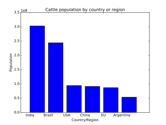
Take a look at the following plot of cattle populations by country, which was generated by a Python program using Matplotlib on an older computer.

Try and run the cattlepopulations.py file yourself. Does the output you see look the same as the one above? If not, why not?

Solution

Matplotlib changed its default style set with version 2.0, so the colours of plots made with the default styles changes between the old and new versions. Also, the default behaviour of bar charts is to centre the labels, where to achieve this before you needed to do extra work.

This is why we must specify our environment when we share our code—otherwise, other people will get different results to us. In this case it was just the formatting of a plot, but in some cases it will be the actual numerical results that will differ!

As an aside, in fact there have been other changes to bar charts so that they are easier to make. Specifically, the positions variable is no longer necessary at all, you can use:

plt.bar(countries, cattle_numbers)

and achieve the same results as the file above did.

Containers

A popular, but somewhat more involved, alternative to using these kinds of environment is to use containerisation, with products such as Docker and Apptainer (previously Singularity). This is beyond the scope of what we’re covering in this lesson, but the Carpentries Incubator provides an excellent lesson on getting started with Docker that is worth looking at if you are interested.

Define another environment

Create a new Conda environment with just the packages you need for the challenge repository, and export an environment.yml file. How long is this file compared to the one for the base Anaconda environment?

Solution

Since this analysis includes running a Jupyter notebook, we need to have Jupyter installed in addition to the packages that are imported in our code.

$ conda create -n challenge
$ conda activate challenge
$ conda install numpy matplotlib pandas jupyter
$ conda env export -f environment.yml

The environment for the challenge repository’s requirements should have around 125 lines, while the full Anaconda environment is over 300 lines.

Using pip and requirements.txt

Try and create an environment for the challenge repository that installs packages via pip and export it to a requirements.txt file.

Solution

Firstly, create a new Conda environment with just Python.

$ conda create -n challenge_pip python=3.9
$ conda activate challenge_pip

Now, install Python packages only using pip, not with conda.

$ pip install numpy matplotlib pandas jupyter

~~ {: .language-bash}

If your project depended on non-Python packages (for example, recent versions of CMake or GNU Make), then you could still install these from Conda.

Now, to export a requirements file:

$ pip freeze > requirements.txt

We could still use conda env export here to generate an environment.yml file, and it would list our packages installed from pip, under a specific entry designating that they were installed via pip.

Key Points

• Different versions of packages can give different numerical results. Documenting the environment ensures others can get the same results from your work as you do.

• pip freeze and conda env export give plain text files defining the packages installed in an environment, and that can be used to recreate it.