Get it in Git

Overview

Teaching: 45 min
Exercises: 25 min

Questions

• Why should I make my code public?

• How do I get files into a GitHub repository?

• What should I include in a repository?

Objectives

• Understand the many reasons for publishing analysis

• Be able to add files to a Git repository and push it to GitHub

• Be able to categorise files into those to commit, and those to omit

Once upon a time, research was published entirely in the form of papers. If you performed a piece of analysis, it would be done by hand in your research notebook or lab diary, and carefully written up, so that anyone with a little time could easily reproduce it. All relevant data were published as tables, either in the main text, or in appendices, or as supplementary material.

Then, computers were invented, and gradually researchers realised that they could get analyses done much more quickly (and with much larger data sets) if they got the computer to do the analysis instead. As time has gone on, computers have got more powerful, and researchers have got more experience of software, the complexity of such analyses has increased, as has the volume of data they can deal with.

Now, since computers are deterministic machines, that (should) always give the same output given the same input, then one might expect that as this occurred, then the ability of other researchers to reproduce exactly the computations that were done to produce a paper has increased. Unfortunately, the opposite has happened! As the complexity of the analysis has increased, the detail in which it is described has not done the same (possibly even gone down), and in most fields it did not immediately become common to publish the code used to produce a result along with the paper showing the result.

This is now starting to change. There has been increasing pressure for some time to publish datasets along with papers, so that the data that were collected (in many cases at significant investment of researcher time or money) are not lost, but can be studied by others to learn more from them. More recently, the same pressure has turned its focus on the software used.

In this lesson, we are going to learn how we can take code that we have written to perform the data analysis (or simulation, or anything else) for a paper, and publish it so that others are able to reproduce our work. We will focus on Python, since that is a popular programming language in research computing, but many of the topics we cover will be more broadly applicable.

Reproduce?

The word “reproduce” here is being used with a specific meaning: another researcher should be able to take the same data, and apply the same analysis, and get the same result. This is distinct from: “replicability”, where another researcher should be able to apply the same analytical techniques to a fresh, different data set, and still get the same results; “robustness”, where applying different analytical techniques to the same data give the same result; and “generalisability”, where applying different analytical techniques to freshly-collected data give the same result.

Reproducibility is in principle the simplest of these to achieve—since we are using deterministic machines, it should be achievable to repeat the same analysis on the same data. However, there are still challenges that need to be overcome to get there.

The Turing Way has more detail on these definitions.

Alternatives

The workflow we will talk about in this lesson is one way to publish code for data analysis—and in many cases is the shortest path we can take to get to a publishable results. In some cases there are other alternative technologies or ways of doing things, that would take a bit longer to learn but could also be very useful. In the interests of keeping this lesson a reasonable length, and because entire lessons already exist about many of these topics, these will be signposted in callouts to where you can learn more.

A first step

In general, we want to do the best job we can; in the context of publishing a piece of data analysis code this means having it run automatically, always give fully reproducible output, be extensively tested and robust, follow good coding standards, etc. However, it is important to not let the perfect be the enemy of the good! Even if we could devote all our time to polishing it, there would always be some area that could be improved, or tidied, or otherwise made slightly better before we called the code “ready” to be published. Add on the fact that we need to keep doing research, and teaching, and in fact can’t devote all our time to polishing one piece of analysis code, and it becomes clear that if we wait until we have all our software in a perfect state before sharing it, then it will never be shared.

Instead, we can take a more pragmatic approach. If the alternative is publishing nothing, then any step we can take towards our goals will be progress! We can start with the absolute minimum step, and work incrementally towards where we’d ideally like to be.

Remember that you were going to publish results based on the code anyway, then the code must already be good enough to trust the output of, so there should be no barrier to making it available.

Difficulties in reproduction

Have you ever tried to reproduce someone’s published work but not been able to, as their publication didn’t give sufficient detail? Would this have been helped if they had published the software they used?

Are there any other situations where your research would have benefited from access to someone else’s analysis code?

Discuss with a neighbour, or in breakout rooms.

Why not publish?

What reasons might there be to be reluctant to publish your data analysis code?

What counterarguments might one have to these reasons?

Discuss with a neighbour, or in breakout rooms.

The first step we will take today is to get your code into version control, and uploaded to GitHub. This will be useful in many ways:

• We can track the history of our analysis as it has developed
• We can share the repository with collaborators and get their input
• We will have a backup version in case we make unwanted changes, or lose data (e.g. a broken or stolen laptop)
• We will be able to connect it to Zenodo later in the lesson to turn the code into a citable object with a DOI

(If you’re already using version control for your analysis code, then you’re already in a strong starting position!)

Let’s start off by opening a Unix shell, and navigating to the example code we will be working on for this lesson.

$ cd ~/Desktop/zipf

Next, we turn this directory into a Git repository:

$ git init

Before we start adding files to the repository, we need to check a couple of things. While most problems we can come back to and fix later (in the spirit of working incrementally), there are a couple of things that are easier to avoid than they are to repair later:

• We do not want to put private or secret data into our repository. Remember that Git stores the complete version history, so even if you remove the secrets in a later commit, they will still be visible to anyone who has access to the full repository. A common problem here is people posting their private tokens for cloud services; there are robots that watch every new upload to GitHub to take any such tokens that get accidentally included, so that they can take over the account and use it for their own nefarious purposes.
• It’s a good idea to avoid putting any large data files into the repository. This means that it’s possible for others to take a local copy of the repository to look at the code without needing to download a large volume of data that they don’t need. Again, even if you later added a commit removing the data, it would still be there in the commit history, so would need to be downloaded every time someone took a fresh copy of the repository.

Let’s see what we currently have:

$ ls

book_summary.sh    dracula.txt        id_rsa             script_template.py
collate.py         frankenstein.txt   id_rsa.pub         utilities.py
countwords.py      full_data.npy      plotcounts.py

Of these, full_data.npy is a few megabytes in size, much larger than any of the code we are working with, so we will omit that. id_rsa is a private SSH key, so that definitely doesn’t want to be committed—it probably ended up in this directory by accident. frankenstein.txt is a piece of data we would like to operate on—since it is small, there are arguments both ways as to whether to keep it in the repository or to publish it separately as data. For now, let’s keep it in; we can always remove it later. (We’ll talk a little more about data later in the lesson.)

Since we don’t want to move or remove files from our existing analysis (which assumes files are where they are currently are placed), we can use a .gitignore file to specify to Git what we don’t want to include.

$ nano .gitignore

*.npy
id_rsa
id_rsa.pub

More to ignore

While we’re creating a .gitignore anyway, you could also add some other common things to make sure not to include in a repository, for example:

• Temporary files, which were used as part of the analysis but are not needed
• Cache files, like __pycache__, that Python sometimes generates, since these are useless on anyone else’s computer
• Duplicate or old copies of code, since we’ll be using Git to manage the history of the code from now on.

GitHub has a repository of common .gitignore files for various languages and technologies that you may want to borrow from.

Now, a check of git status will show us what Git would like to commit:

$ git status

On branch main

No commits yet

Untracked files:
  (use "git add <file>..." to include in what will be committed)
	.gitignore
	book_summary.sh
	collate.py
	countwords.py
	dracula.txt
	frankenstein.txt
	plotcounts.py
	script_template.py
	utilities.py

nothing added to commit but untracked files present (use "git add" to track)

To get all of these files into an initial Git commit, we can add them to the staging area and then commit the resulting data:

$ git add .
$ git commit -m 'initial commit of analysis code'

Finally, we need to push this to GitHub. Visit GitHub and create a new, empty repository. In this case, let’s call the repository zipf-analysis. Add this repository as a remote to your local copy, and push:

$ git remote add origin git@github.com:USERNAME/zipf-analysis
$ git push origin main

SSH keys

If you find that GitHub doesn’t let you do this, then you will need to set up key authentication with GitHub. To do this, follow the instructions in the Software Carpentry Git lesson.

We now have the code that we used for our research stored online, and available. If we had no more time, we could put a footnote pointing to this repository, and call it done. However, with a little extra effort, there are many ways we can improve on this, and as we go through the remainder of the episode we will see how.

What to include

Anneka has a folder containing the analysis that she has performed, and that she is preparing to publish as a journal article. It contains the following files and subfolders:

• fig5.py, which plots a graph used in the paper draft
• A folder called __pycache__; Anneka isn’t sure what this is
• analyse_slides.py, which doesn’t generate anything included in the paper directly, but generates numbers needed by fig5.py
• table3.tex, an output file used in the publication
• A folder called tensorflow containing the source code for the TensorFlow library, which Anneka needed to manually install
• participants.csv, a listing of the people that Anneka took samples from, and which images are from which person.
• Makefile, which Anneka got from a collaborator; she isn’t sure what it does
• test.py, which doesn’t generate any outputs used in the publication, but does illustrate a simple example of how to use the code
• .DS_Store and thumbs.db, which keep showing up on Anneka’s disk
• fig5_tmp.py, which was used by Anneka to test some modifications to one of the graphs in the paper but was ultimately not used for the final analysis

Which of these (if any) should Anneka include in her repository? In each case, why, or why not?

Solution

• fig5.py: This is needed to reproduce Anneka’s work, so should be included.
• __pycache__: This is a folder you will frequently see when working with Python; it contains temporary files generated from your Python code by the Python interpreter. It is useless on anyone else’s computer, so should be excluded.
• analyse_slides.py: Even though no outputs are used directly in the publication, this file is needed to reproduce Anneka’s work, so should be included.
• table3.tex: This should be generated as an output of the code, and is included as part of the publication, so doesn’t need to be included in the repository.
• tensorflow: The source code to Tensorflow is available elsewhere, so should not be included in the repository. We’ll discuss later how to specify what packages need to be installed for your analysis to work. Note that if Anneka has made changes to Tensorflow, then these should be in a repository, but probably not this one—Tensorflow is much larger than the analysis for one paper, and has its own repository. Look up the idea of “forking on GitHub” for more information about one way this could be done.
• participants.csv: This is data, not code, so we would need to decide whether we are mixing data and code, or keeping this repository to be code-only. Since it is also personal, private data, special care would need to be taken before this is committed to any public repository, either for data or code.
• Makefile: Anneka should understand what this does before committing it. It’s possible that she is using it without realising it (e.g. if she runs Make), in which case it is needed to reproduce her work. Perhaps she could check with her collaborator what the Makefile does.
• test.py: While not strictly necessary to reproduce Anneka’s work, this file could help someone else looking to do so to better understand how Anneka’s code works. It’s not essential to include, but committing it is probably a good idea.
• .DS_Store and thumbs.db: These are metadata files made by macOS and Windows; they’re useless on anyone else’s computer, and should not be committed.
• fig5_tmp.py: Since there is already a canonical version of fig5.py above, this alternative version should not be committed.

Creating another repository

Download this example archive of code and extract it to a convenient location on your computer. This will give you a directory containing a small piece of research software, and the data it was last used to analyse.

Turn this directory into a repository and push it to GitHub.

Remember to exclude any files that shouldn’t be in the code repository.

FAIR’s fair

You might have heard of the concept of “FAIR data”, and more recently “FAIR software”. The acronym FAIR stands for:

• Findable
• Accessible
• Interoperable
• Reusable

The standards for data are well-developed; the situation for software (i.e. code) is more fluid, and still continuing to develop. For this lesson, we will address the first two points; the latter two points are a step further—the aim for now is to let us document what we have done in our own work, rather than provide tools for others to use.

In the spirit of not letting the perfect be the enemy of the good, this lesson is doing what it can for now; as standards develop, it may be updated.

Key Points

• Publishing analysis code allows others to better understand what you have done, to verify that your analysis does what you claim, and to build on your work.e

• Use git init, git add, git commit, git remote add, and git push, as discussed in the Software Carpentry Git lesson

• Include all the code that you have written to use in this analysis.

• Leave out e.g. temporary copies, old backup versions, files containing secret or confidential information, and supporting files generated automatically.

Structuring your repository

Overview

Teaching: 40 min
Exercises: 20 min

Questions

• How should files be organised in a repository?

• What metadata should be included, and how?

• How do I adjust the structure of a repository once it is created?

Objectives

• Be able to organise code, documentation, and metadata into an easy-to-user directory layout.

• Understand the importance of a README, license, and citation file.

• Be able to restructure an existing repository.

Now that we have a repository to work with, and that has all of our code in, we can start tidying it up so that it is easier for others to understand.

README

A README is the first thing you should add to your repository, if it doesn’t already have one. The file name convention is old—it dates to before you could have lower case letters and spaces in a file name—and is intended as an instruction to anyone who happens upon it to read it before looking anywhere else. READMEs were originally (and frequently still are) plain text files, although other formats are also popular now.

Markdown

A popular format for READMEs on GitHub is Markdown, which looks like plain text but specific characters will let you indicate headings, bold, italic, etc.

For more information about Markdown, you might check out the Carpentries Incubator’s Introduction to MarkDown.

Conversely, when you start using a new piece of software (or investigate someone else’s analysis code), it’s a good idea to start by looking for a README to see what the author thought was important you understand first.

There are many things that you can include in a README. Exactly what should and shouldn’t go there will depend on your project, and don’t forget that starting with something short is still better than having no README at all. (On the other hand, a README that is incorrect can be less helpful than no README at all, so be sure to keep yours updated if your code changes.) Some things to consider

• The name of the code, or project; this typically goes at the top
• A short description of what the code does
• A link or citation to the paper (or a preprint) the work supports, if it is available
• Instructions on how to install and use the software (which we’ll discuss in more detail in a later episode)

Let’s write a short README for the zipf repository now.

$ cd ~/Desktop/zipf
$ nano README.txt

zipf analysis
=============

This repository contains code to observe whether books adhere to Zipf's law, as
done in support of the paper "Zipf analysis of 19th-century English-language books",
V. Dracula, to appear in Annals of Computational Linguistics, 2022.

To run the code, you will need the Pandas package installed.

This is a little brief, but is some progress, and we’ll revisit tightening up some of the details in later episodes.

Let’s commit this to the repository now.

$ git add README.txt
$ git commit -m 'add a README'
$ git push origin main

We’ll be keeping up this habit of regularly committing and pushing, so that our fallback version on GitHub stays up to date. (The benefits of storing a copy remotely are lost if when your laptop is stolen you have to fall back on a version from years ago!)

LICENSE

The next thing to do is to let people know what they’re allowed to do with your code. (Or, conversely, what they’re not allowed to do!) By default, copyright law is a huge barrier to doing anything productive with code that is not explicitly licensed.

Since we are researchers, not copyright lawyers, writing our own license from scratch is not a good idea. It’s more likely that we will either not give away the permissions we need for someone to be able to use the code, or give away rights that we do not intend to. (Or both.) It’s much safer to pick a license that someone else has designed, and that has been written and vetted by teams of copyright lawyers. This has the added bonus of being more widely understood; someone reading a set of rights you’re giving explicitly will be more confused than if they saw the name of a familiar license, and if they have a particularly careful legal department, then they’ll be much happier to see a familiar name.

A good place to start when deciding what license to give to your research code is Choose a license, which has a comparison table of some of the more common licenses used for software. Some questions to ask yourself:

• Do you want others to have to share their changes to your source code under the same terms if they share the software?
• Do you want others to be able to distribute your code under the same name (trademark rights)?
• If your code makes use of patents you own, are you giving users of the code rights to use them?
• Do others need to explicitly state what changes they’ve made to your version?
• Can others run your software as a service without sharing changes?

Let’s place Zipf under the MIT License.

$ nano LICENSE

MIT License

Copyright (c) 2020 Amira Khan, Ed Bennett

Permission is hereby granted, free of charge, to any person obtaining a copy of this software and associated documentation files (the "Software"), to deal in the Software without restriction, including without limitation the rights to use, copy, modify, merge, publish, distribute, sublicense, and/or sell copies of the Software, and to permit persons to whom the Software is furnished to do so, subject to the following conditions:

The above copyright notice and this permission notice shall be included in all copies or substantial portions of the Software.

THE SOFTWARE IS PROVIDED "AS IS", WITHOUT WARRANTY OF ANY KIND, EXPRESS OR IMPLIED, INCLUDING BUT NOT LIMITED TO THE WARRANTIES OF MERCHANTABILITY, FITNESS FOR A PARTICULAR PURPOSE AND NONINFRINGEMENT. IN NO EVENT SHALL THE AUTHORS OR COPYRIGHT HOLDERS BE LIABLE FOR ANY CLAIM, DAMAGES OR OTHER LIABILITY, WHETHER IN AN ACTION OF CONTRACT, TORT OR OTHERWISE, ARISING FROM, OUT OF OR IN CONNECTION WITH THE SOFTWARE OR THE USE OR OTHER DEALINGS IN THE SOFTWARE.

Names

You might have spotted that the name in the README doesn’t match the name in the license here. This is because the paper referred to in the README is imaginary, while the code is actually written by real people and licensed by them, so we need to acknowledge them appropriately, even on a toy example project like this.

Again, let’s commit and push:

$ git add LICENSE
$ git commit -m 'add a LICENSE'
$ git push origin main

CITATION

The idea of a CITATION file is much newer than the README and LICENSE, and the uppercase is a convention carried over from the latter two rather than ever having been technically necessary. It is rather more specific to software used in an academic context.

In its simplest form, the CITATION file should describe how someone who finds your code useful in their own research (in particular, but not only, if they use/modify it themselves to generate their own results) should cite it. Sometimes this will be a citation to the paper that the code supports, but we’ll discuss later how the repository itself can be cited in the final episode.

In the absence of a CITATION file, many researchers using your work may instead use a footnote with a URL, or text in the acknowledgement, or some other way that makes it much harder to track how much impact your work is having. While assessing work on the basis of citation counts is fundamentally flawed, citation is still a vital part of good scholarship, and having clear and consistent data on what work is being referred is both invaluable in itself and also a vital part of intellectual honesty—as Newton said, we are only able to research by standing on the shoulders of giants.

For now, we can add a brief text description of how to cite the work.

$ nano CITATION

If you use this code in your own work or research presented in a publication, we ask
that you please cite:

"Zipf analysis of 19th-century English-language books",
V. Dracula, to appear in Annals of Computational Linguistics, 2022

Again, we should now commit and push this:

$ git add CITATION
$ git commit -m 'give information on how to cite'
$ git push origin main

Citation file formats

If you are in a field that makes use of LaTeX, you may consider including a BibTeX version of your citation so that others can copy it directly into their work.

There is also a Citation File Format, which lets you specify citation information in a more structured format.

Directory structure

Now that we’ve started adding metadata to the repository, the root directory is starting to get a little cluttered. For someone arriving at the repository for the first time, it might be hard to tell what is important information they need to look at, what is the code that they need to run first, and what is ancillary supporting code that they can dig into at a later date.

To make this easier, you should use directories (folders) to separate out related elements. Things like the README, LICENSE, and CITATION, that apply to the whole repository (and that users will need to see first) should be at the root of the repository. Code should go in its own subdirectory—by convention this is called bin.

bin and src

Like most conventions, there are alternatives to the bin directory. Another common alternative is to use a src directory. For Python packages specifically, you may also see a directory with the same name as the repository

If you have a lot of code, then it might be a good idea to split it up. A directory with dozens or hundreds of files in is not conducive to easy reading! Again, grouping related files together is the target—for example, you could group all of your figure files in one directory, files with common functionality that are never called directly from the command line in another.

Let’s rearrange the files in the zipf repository now. We can do this using the git mv command. This moves a file in the same way that mv does, but also alerts Git about the change so that it can be committed more easily.

$ mkdir bin
$ git mv *.py *.sh bin

The frankenstein.txt looks to be data that the code operates on. This doesn’t belong in the same directory as the code, and neither does it belong in the root of the repository. Let’s give it its own data directory for now.

$ mkdir data
$ git mv frankenstein.txt dracula.txt data

Now that this is done, we also need to change the programs that expect to see these files:

$ nano bin/countwords.py

with open('data/frankenstein.txt', 'r') as reader:

Now we can add this change to the repository, and commit the full adjustment to the directory structure.

$ git add bin/countwords.py
$ git commit -m 'reorganise directory structure'
$ git push origin main

As our repository is small we’ve done this reorganisation in a single step, but of course if there were more to do we could do things in stages, working incrementally.

Python packaging

You can take this structure to the next level with the concept of a Python package. This is a specific structure designed so that others can install your repository and have it accessible via import like other packages you might install with pip.

For just publishing your analysis this can be overkill, but if you think any of the code you have written could be useful more generally, then packaging it is a very good idea. While it’s too much for the time we have this week, the (free, online) book Research Software Engineering with Python has a section on Creating Packages with Python.

Tidying up

Kazu has committed his analysis directory into a Git repository. While he is happy that he now can keep track of versions and share with colleagues, he realises that to allow others to easily make use of the workflows he’s prepared, he will need to make some improvements to the structure of the repository.

Given the structure below, what changes would you suggest Kazu make?

analyze.py
draw_fig3.py
fig1.py
figure_2.py
notes/
  notes_for_julia.eml
tables_code.zip
test.py

Solution

Some things that Kazu might want to consider (there may be others!):

• fig1.py, figure_2.py, and draw_fig3.py could be renamed consistently
• The .py files could be placed in a bin subdirectory
• Code isn’t very useful in a ZIP file; it would be better if the programs in this file were committed directly to the repository instead
• The notes_for_julia.eml looks like it might be the only documentation Kazu has written for this code. Perhaps it could form the basis of a README. This should be in the root of the repository, and probably shouldn’t be in the form of an email.
• analyze.py could also be in the bin directory. Kazu might also want to have subdirectories of bin specifically for analysis, plots, and tables.
• Kazu should specify licensing and citation information.

Choosing a license

Kai has written some engineering analysis code that could be very useful in the private sector. They don’t like the idea of their hard work being used as the basis for a commercial product that they won’t see any income from (especially if they start to receive requests for support), so they would like a license that makes sure that any changes to the software are made freely available, and with the same rights to those who receive the modified version.

Sameth has prepared some code for genetic analysis that solves a very specific problem, but that others with more financial resources may also be able to adapt to do some very impactful research that could form the basis of an Impact Case Study. Due to the way the field works, these others would need to be able to distribute the software, but would want to prevent others from seeing or redistributing their modified versions.

What licenses would you suggest that Kai and Sameth choose for their software?

Solution

Kai is most likely looking for the Affero GNU Public License, although they may instead opt for the GNU Public License.

Sameth could use the MIT or BSD license, among others.

If no-one else contributes changes back to their code, then nothing is stopping them negotiating a separate licensing agreement—for example, if a major engineering firm wanted to pay Kai for the rights to distribute modified versions without sharing the code. However, Kai would need to be careful about who owns the code—if they are a postdoc, then it may be their university who has the rights to this.

If others have also made contributions, then whether you can re-license the code will depend on getting the agreement of all authors. A Contributor Agreement makes this easier, by granting certain rights up-front rather than needing to track down a lot of authors later.

Tidy up for yourself

In the previous episode’s challenges, you created a challenge repository for the example code downloaded. Use git mv now to start tidying up this repository.

Solution

$ mkdir bin data results
$ git mv calc_fractal.py fig?.py bin/
$ git mv survey.csv data/
$ touch results/.git_keep
$ nano bin/calc_fractal.py
$ # edit calc_fractal.py to place the output in the results/ directory
$ nano bin/fig1.py
$ # edit fig1.py to use data from the results/ directory
$ nano bin/fig2.py
$ # edit fig2.py to use data from the results/ directory
$ nano bin/fig3.py
$ # edit fig3.py to use data from the results/ directory
$ nano bin/fig4.py
$ # edit fig4.py to use data from the data/ directory
$ git add bin results
$ git commit -m 'tidy directory structure'

Key Points

• Put code into a specific subdirectory (or several, if there is lots of code).

• Keep important metadata, such as a license, citation information, and README in the root of the repository.

• Keep other ancillary data, documentation, etc. in separate subdirectories.

• Use git mv to move files and let Git know that they have moved.

Documentation and automation

Overview

Teaching: 60 min
Exercises: 25 min

Questions

• How do I tell other researchers how to use my code?

• How can I make it easier for others (or me) to run my full analysis?

Objectives

• Be able to write a README documenting how to run a tool.

• Be able to write a shell script to automate an analysis process.

• Understand how to remove manual editing steps from processes.

Sharing your code and giving it a comprehensible structure is a great first and second step, but without some guidance on how to run your code, then others will find it very difficult to reproduce your steps. To you it might be obvious that you first run incomprehensible_longname.py and then another_long_name.py, but it likely won’t be to anyone else.

Thus, we need to make sure to explain to others how to make use of the code that you have shared with them. There are two main ways to do this: descriptively, and programmatically.

Describing in English (or your preferred human language) how to use the software has the advantage that you can do it relatively quickly, from memory, and with little testing, since the “code” you are writing runs on a human brain, which can figure things out if they are unclear. The disadvantage is that you can’t do very much testing; you don’t know how someone else will interpret your instructions. Conversely doing things programmatically so that the complete analysis is fully automated takes more effort up front, but again makes it even easier to run your code.

To start with, let’s see what a descriptive README of the zipf project might look like.

To reproduce the figures in the publication, follow these steps:

1. Create a `results` directory

2. Use `countwords.py` to count the words in `frankenstein.txt`.

      python bin/countwords.py > results/frankenstein.csv

3. Use `plotcounts.py` to plot the resulting file.

      python bin/plotcounts.py

4. Save the plot as `results/frankenstein.pdf`.

5. Edit `bin/countwords.py` and `bin/plotcounts.py` to replace `frankenstein` with `dracula`.

6. Repeat the above instructions to generate `dracula.csv` and plot `dracula.pdf`.

Let’s commit this:

$ git add README
$ git commit -m 'add run instructions to README'
$ git push origin main

Once again, these instructions are substantially better than what we had before. Then, we would have had to pore over the code to work out what it did, and guess at what exactly was done. If you have time to write this but not to do more work to automate the analysis, then it is definitely work worth doing.

Does it work?

Try following the instructions in the README above. Do they work? If not, then try and identify what is causing the failure, and fix it. If you get stuck, ask a helper for support.

Avoid manually editing parameters

While having instructions is good, it would be good if we could remove at least some of the manual effort from this process.

The most obvious issue here is that it is rather laborious to have to edit a source file in order to change which analysis is done. This is very error-prone, and risks others getting different results to you and challenging your work (or worse, you making an error in your own work and needing to revise your results after publication). In this project you may end up with the wrong book name on a figure; in others the parameters may be numbers, so the error may become even more difficult to spot.

To avoid this, we would like our programs to take command-line arguments rather than having parameters hard-coded. We saw in Software Carpentry one way of doing this, by using sys.argv. That works, but can be a little fragile. Instead, here we will introduce the argparse module from the Python standard library; this gives a way of defining in more depth what arguments you want your program to accept.

This is slightly more verbose than using sys.argv directly, but gives an improvement in usability that makes it more than worthwhile.

Let’s start with countwords.py. To begin, we add argparse to our imports at the top of the file.

$ nano bin/countwords.py

import argparse

Now, where we want to start doing work, we will create an ArgumentParser, specify what arguments we want it to accept, and then parse them out from our input.

parser = argparse.ArgumentParser(description=(
    "Count the occurrences of all words in a text "
    "and write them to a CSV-file."
))
parser.add_argument('infile', type=argparse.FileType('r'),
                    nargs='?', default='-',
                    help='Input file name')
parser.add_argument('-n', '--num',
                    type=int, default=None,
                    help='Output only n most frequent words')
args = parser.parse_args()

Working through this line-by-line:

• We create an ArgumentParser, giving it a description of what our program does.
• We add the infile argument, which will give us a file. If no argument is specified, then the default value is used, which in this case means “read from standard input”. We also give it a description.
• We add the --num optional argument, which can also be referred to more briefly as -n, will be interpreted as an integer, defaults to None, and has a help message.
• We use all of this to interpret the command line that the program was run with.

Finally, we can use args.infile instead of needing to use open(), since argparse handles the file opening by itself. We then use args.num in place of the hard-coded 100.

word_counts = count_words(args.infile)
util.collection_to_csv(word_counts, num=args.num)

We can now check that the analysis described in the README still works, once the function names are adjusted.

$ python bin/countwords.py data/frankenstein.txt --num 100 > results/frankenstein.csv
$ python bin/countwords.py data/dracula.txt --num 100 > results/dracula.csv

Currently the README is no longer correct, since the program doesn’t automatically look for frankenstein.txt any more. So, let’s hold off committing it for now.

More argparse

argparse has a huge array of options, which is too detailed to go into here.

Check out the argparse documentation to find out more.

argparse alternatives

argparse is far from the only way to parse command-line arguments; there is a variety of packages available. One popular alternative is Click, which makes use of function “decorators” to define commands and arguments. If you see functions when reading others’ code that contain lines like

@click.command()

above function definitions, then this code is making use of Click. You can read more about Click at the Click documentation.

Try it yourself

Get the plotcounts.py program to also use argparse. Allow the user to specify the xlim argument to scatter in addition to the infile.

Solution

parser = argparse.ArgumentParser(description="Plot word counts")
parser.add_argument('infile', type=argparse.FileType('r'),
                    nargs='?', default='-',
                       help='Word count csv file name')
parser.add_argument('--xlim', type=float, nargs=2,
                    metavar=('XMIN', 'XMAX'),
                    default=None, help='X-axis limits')
args = parser.parse_args()

df = pd.read_csv(args.infile, header=None,
                 names=('word', 'word_frequency'))
df['rank'] = df['word_frequency'].rank(ascending=False,
                                       method='max')
df['inverse_rank'] = 1 / df['rank']
ax = df.plot.scatter(x='word_frequency',
                     y='inverse_rank',
                     figsize=[12, 6],
                     grid=True,
                     xlim=args.xlim)
plt.show()

Avoid interactivity

The next biggest issue with this software is that you have to manually save the plot output. This is common in tools used interactively for data exploration, but once you’re publishing your analysis then it makes more sense to save to a file directly from the program.

This isn’t a huge change. In most cases, we can replace plt.show() with plt.savefig(filename). If we are generating multiple plots we will need to be more careful, as savefig doesn’t start a new plot in the way that show() does.

Looking at plotcounts.py, we can also avoid hardcoding the filename to write by adding an extra argument to the ArgumentParser.

parser.add_argument('--outfile', type=str,
                    default='plotcounts.png',
                    help='Output image file name')

Note that now we don’t use the FileType, since we don’t want argparse to open the file—Matplotlib does this for us, so we just need a filename.

Now, we replace the last line with

plt.savefig(args.outfile)

Since the program is ending anyway, we don’t need a plt.close() here.

Checking again that our code still works after this modification:

$ python bin/plotcounts.py results/frankenstein.csv --outfile results/frankenstein.pdf
$ python bin/plotcounts.py results/dracula.csv --outfile results/dracula.pdf
$ ls -l results

total 72
-rw-r--r--  1 ed  staff    963  6 Apr 16:45 dracula.csv
-rw-r--r--  1 ed  staff  13071  6 Apr 16:50 dracula.pdf
-rw-r--r--  1 ed  staff    948  6 Apr 16:45 frankenstein.csv
-rw-r--r--  1 ed  staff  12245  6 Apr 16:50 frankenstein.pdf

Your output will differ, but should show both PDF files modified in the last minute or so.

Avoid bare code

Frequently we define functions in Python files. In order to import these into other pieces of Python code, Python runs the entire file top-to-bottom.

The effect of this is that if there is any code not within a function (or other block that would prevent it doing so), then it will automatically run when we import the module. For example, in countwords.py, the word count would be run even if we didn’t want it to be.

As such, you will frequently see guards of the form if __name__ == '__main__' in programs. This checks to see whether the Python file is being run directly as a program, or imported into another file as a module. These aren’t always needed—in larger programs many programmers will try to keep “tools” that can be run by the user entirely separate from shared libraries that get imported. But in the kinds of code written for research they are frequently useful.

Let’s update countwords.py now:

def main(args):
    """Run the command line program."""
    word_counts = count_words(args.infile)
    util.collection_to_csv(word_counts, num=args.num)


if __name__ == '__main__':
    parser = argparse.ArgumentParser(description=(
        "Count the occurrences of all words in a text "
        "and write them to a CSV-file."
    ))
    parser.add_argument('infile', type=argparse.FileType('r'),
                        nargs='?', default='-',
                        help='Input file name')
    parser.add_argument('-n', '--num',
                        type=int, default=None,
                        help='Output only n most frequent words')
    args = parser.parse_args()
    main(args)

Try it yourself

Adjust the plotcounts.py file to use if __name__ == '__main__' guards.

Check that it still works correctly afterwards.

Use a shell script

The final step (for this lesson at least) in documenting your analysis through automation is to write a shell script that will run all the steps needed in turn.

Now that we have adjusted the tools to not need direct interaction, this becomes relatively short:

$ nano bin/run_analysis.sh

mkdir -p results
for book in dracula frankenstein
do
    python bin/countwords.py data/${book}.txt --num 100 > results/${book}.csv
    python bin/plotcounts.py results/${book}.csv --outfile results/${book}.pdf
done

Now we can edit the README again:

To reproduce the figures in the publication, run the command:

    bash bin/run_analysis.sh

Results will be placed in a `results/` directory.

Before we commit this, let’s check that it works!

$ bash bin/run_analysis.sh
$ ls -l results

total 72
-rw-r--r--  1 ed  staff    963  6 Apr 16:55 dracula.csv
-rw-r--r--  1 ed  staff  13071  6 Apr 16:55 dracula.pdf
-rw-r--r--  1 ed  staff    948  6 Apr 16:55 frankenstein.csv
-rw-r--r--  1 ed  staff  12245  6 Apr 16:55 frankenstein.pdf

Now both CSV and both PDF files should all be modified within the last minute or so.

As the README and the code are now consistent and working, we can commit this:

$ git add bin/countwords.py bin/plotcounts.py bin/run_analysis.sh README.txt
$ git commit -m 'automate analysis'
$ git push origin main

Note that for the sake of simplicity today we have done this as a single pass, but we could just as well have done this in smaller steps. We could update one tool to be easier to run automatically, adjust the README to match, commit, push. Then move on to the next one, and so on, until we get to the point we have now reached.

Empty directories

We had a shell script here create the results directory. Sometimes it is convenient to provide an empty directory, rather than having to create it. Since Git only stores files, not directories, by convention this is done by placing a hidden file called .git_keep into the directory and adding it to the repository.

$ mkdir results
$ touch results/.git_keep
$ git add results/.git_keep
$ git commit -m 'add an empty results directory'
$ git push origin main

Truths about READMEs

Take a look at the following statements. Which do you think are true?

1. If I write a good enough README, then I’ll never need any other documentation
2. If I write a shell script that does my entire analysis, I don’t need a README
3. If I don’t have a README, my repository is useless.
4. A README should have instructions on using the software, and information on what it does.
5. A README should be plain text only. Other documentation can have more formatting.

Solution

1. False. While a good README may be enough documentation for a very small project, more frequently you will benefit from other types of documentation; for example, comments in your code, and more detailed descriptions for more technical aspects.
2. False. Even if a shell script completely reproduces your outputs, you should have a README to point the user at the right script to run, and to describe what to expect.
3. False. Having your code in version control and shareable is a good step! But without a README, it’s likely that others will find your code hard to use or understand. (As will you if you return to it after a few months or years!)
4. True. Normally the ordering is reversed, though, with the description of the purpose of the code coming before the details on using it.
5. False. Historically READMEs were plain text files, but now they take a variety of formats; many will use Markdown, which allows headings, bold, italic, images, etc.

make it better

A more powerful alternative to using shell scripts to document and automate your analysis process is to use a workflow management tool. A simple one of these that is frequently used in software development is called Make; Software Carpentry has a lesson on getting started with Make.

More powerful again are tools like Snakemake and Nextflow, which are used for very intricate scientific analyses with very many steps.

We don’t have time to look into these tools in more detail in this lesson, but if you find that your shell scripts are getting too long or intricate, then it it might be worth your time to look into using one of these tools.

Removing hardcoded data

Take a look at the calc_fractal.py file in the challenge repository. Currently this will generate the files needed for fig3.py, but must be edited to allow fig1.py and fig2.py to run correctly.

Adapt calc_fractal.py to allow this parameter to instead be set by a command-line argument.

Solution

There are a few ways to do this. One is to use some ifs:

parser = argparse.ArgumentParser()
parser.add_argument('order', type=int, help="Order of the polynomial")
parser.add_argument('outfile', type=str, help="Where to put the output file")
args = parser.parse_args()

if args.order == 3:
    def polynomial(x):
        return x ** 3 - 1

    def derivative(x):
        return 3 * x ** 2
elif args.order == 5:
    def polynomial(x):
        return x ** 5 - 1

    def derivative(x):
        return 5 * x ** 4
elif args.order == 6:
    def polynomial(x):
        return x ** 6 - 1

    def derivative(x):
        return 6 * x ** 5
else:
    raise ValueError(f"I don't know how to handle order {order}.")

This is quite verbose, and repeats itself. If they are familiar to you, you might want to use some more advanced features of Python to reduce the amount of repetition. For example, using dictionaries and lambdas:

polynomials = {
    3: lambda x : x ** 3 - 1,
    5: lambda x : x ** 5 - 1,
    6: lambda x : x ** 6 - 1
}

derivatives = {
    3: lambda x : 3 * x ** 2,
    5: lambda x : 5 * x ** 4,
    6: lambda x : 6 * x ** 5
}

results = angle(
    newton(polynomials[args.order], derivatives[args.order], initial_z, 20)
)

Or using functools.partial:

from functools import partial

def polynomial(x, order):
    return x ** order - 1

def derivative(x, order):
    if order == 0:
        return 0
    else:
        return order * x ** (order - 1)

results = angle(
    newton(partial(polynomial, order=args.order),
           partial(derivative, order=args.order),
           initial_z,
           20)
)

Now, adapt the instructions in the README into a shell script to allow the analysis to be run automatically.

Solution

mkdir -p results
python bin/calc_fractal 3 results/data.dat
python bin/fig1.py
python bin/calc_fractal 5 results/data.dat
python bin/fig2.py
python bin/calc_fractal 6 results/data.dat
python bin/fig3.py
python bin/fig4.py

What other change would be needed to allow this analysis to be run unattended?

Solution

Currently the images are shown on the screen; the user must save and close each image. It would be better to use savefig to save the figure to disk, instead.

Key Points

• Use a README or similar file to explain the essential steps of running your analysis.

• Use shell script or similar to automate the steps you would take to perform your analysis.

• Use command-line arguments or other parameters instead of having to manually edit lines of code.

Jupyter Notebooks and automation

Overview

Teaching: 25 min
Exercises: 20 min

Questions

• How does using Jupyter Notebooks affect automation and reproducibility?

• How do I put a Jupyter Notebook into a repository?

• What changes can I make to a Jupyter Notebook to improve automation?

Objectives

• Understand what data are included in a Jupyter Notebook, and how to remove it

• Be able to adjust notebooks to reduce manual intervention

Since their introduction barely a decade ago, Jupyter Notebooks have become an incredibly popular tool for working interactively with data and code (in particular Python code). The notebook structure means that compared to an interactive Python session, a lot more is saved, and results can be presented contextualised by the code that generated them, and with documentation describing what was done. They are held by many to be a “good thing” for reproducibility. However, they come with some unique challenges that in some cases make reproducibility harder rather than easier! In this episode we will look at what causes some of these challenges, and how we can overcome them.

Run in order

Something you’ve probably noticed when working with Jupyter Notebooks is that you can go back and modify and re-run old cells. Unfortunately, this doesn’t recompute all of the results that had been calculated based on the first run of the cell. This then means that the notebook can get into an inconsistent state, where some variables have “old” data and some are up to date. It would be very difficult for another researcher to re-run the notebook in the same order—they would need to painstakingly look through the little numbers Jupyter attaches to the cells after they are run, finding each one sequentially. And in some cases that wouldn’t be sufficient— for example, if a cell had been edited since the last time it was run.

As an example, let’s look at spiral.ipynb. Since the second cell specifies to draw a spiral, we would expect to see one in the output of the third cell, but instead we see a straight line. Looking carefully, we can see that the second cell was run after the third cell, so presumably the value of line_to_draw was changed.

To avoid this issue, we should always purge the output, restart the kernel, and re-run our notebooks top-to-bottom once we think our analysis is complete, to ensure that the notebook is consistent and does indeed give the answers we want. However, this is laborious, and ideally we would like to automate it. Fortunately, Jupyter gives us a tool to do it:

$ jupyter nbconvert --to notebook --execute spiral.ipynb

The notebook is updated as if we had opened it in the browser and run every cell, but we never had to leave the command line. This would then allow the notebook to be called from a shell script, or any other tool we’ve written to automate our analysis.

Stripping output

There are two reasons one might want to commit a Jupyter notebook to a Git repository:

1. To share the results of an analysis, including the code that generated it for context. In this case, the output is key and needs to be retained as part of the file.
2. To keep track of, or share, the code used, with the intention that others generate the output. In this case, the output is in fact a hindrance.

Why is the output a hindrance in a Jupyter notebook in Git? There are a few reasons: firstly, it makes the file much larger than it needs to be, since there are most likely images (e.g. plots) in it that will take up much more space than the code. Another is that time the notebook is run it will change some aspect of the output (e.g. the cell numbers). This means Git will see the file as changed and suggest we commit it, even if no change has been made to the code we actually want to track.

Manually clearing the output before quitting each Jupyter Notebook session will avoid this, but is difficult to remember every time. More convenient is a tool called nbstripout, which is available from pip.

$ pip install nbstripout

We can now manually strip the output from a notebook with:

$ nbstripout spiral.ipynb

If we want to go a step further, we can even get nbstripout to attach itself to our local copy of the repository, and automatically strip notebook as we commit them, so that we never accidentally commit a notebook with output in.

Git smudge/clean filters

nbstripout is an example of a Git clean filter, which silently adjust files as they are read into a Git repository. Since different people will have tools installed in different places, Git does not pull or push the definitions of filters; instead, each person cloning a repository (or each computer you clone it to) will need to install the filter to their local copy separately.

More detail on how smudge and clean filters work can be found in this article on RedHat.com.

$ nbstripout --install

Of course, if we have a use case where we want to commit notebooks with output, we would not want to install nbstripout in this way. The nbstripout --install command only attaches nbstripout to the current repository, so we can be selective about which repositories get this treatment.

Diff and merge

You may recall that Git has some powerful tools for helping resolve merge conflicts, where you and a collaborator have edited the same file at different times. The structure of a Jupyter Notebook makes this much harder to resolve than it would be for a plain text file. Fortunately, there are is a tool available to help with this, called nbdime. If you will be collaborating with others on a repository that contains Jupyter Notebooks, then reviewing the documentation for nbdime (and installing it) is very much recommended!

More to ignore

When working with Jupyter notebooks, you may have noticed that they generate an .ipynb_checkpoints directory, that clutters the output of git status. We can fix that by adding it to our .gitignore.

Passing arguments to notebooks

Unlike regular Python programs, notebooks can’t take command-line arguments. But we’ve already discussed in the previous episode that we don’t want to have to manually edit code to set the right parameters for the particular analysis we want to perform.

One way of working around this problem is by using environment variables. These are a general feature of most operating systems; we can set variables in a shell and have them accessible within programs running inside that shell.

Environment variables are accessible in Python via the os.environ dictionary. By convention, the names of environment variables are written in all capitals:

import os

print(os.environ)

Let’s say that we would like to adjust the size of the spiral being drawn by spiral.ipynb. We can look for an environment variable called SPIRAL_MAX_X, and if one is found, use that in place of the 20 that we are currently using. We replace the line x = np.linspace(0, 20, 1000) with:

import os

max_x = float(os.environ.get('SPIRAL_MAX_X', 20))
x = np.linspace(0, max_x, 1000)

The .get() method of a dictionary will give us the element corresponding to the key we passed ('SPIRAL_MAX_X'), unless there is no such element, in which case it will return the second parameter (20). Since environment variables are always strings of text, we then need to convert the result into a number so that Matplotlib understands it.

To call this with jupyter nbconvert, we can add the environment variable definitions at the start of the line.

$ SPIRAL_MAX_X=100 jupyter nbconvert --to notebook --execute spiral.ipynb

This will now give us a much tighter spiral.

To notebook or not to notebook

Many computational researchers treat notebooks as a tool for data exploration, or presentation, rather than for reproducibility. They will use notebooks to prototype and find interesting features, before formalising the analysis that has been done into a plain .py file to make the analysis reproducible. These can then be loaded into smaller notebooks as modules to present and highlight particular aspects of the results. If you have the time to do this, it is certainly not a bad workflow, but if you have a large amount of Jupyter Notebooks containing your entire analysis for a paper or thesis, then taking that and porting it back to plain Python files may take more time than you have available, in which case tidying up the notebook and making it more reproducible in and of itself may be more achievable in the time you have available.

Bringing matters to order

Sanjay is investigating some work by his colleage Prof. Nuss, whose conclusions he disagreed with. Prof. Nuss included the following figure in a publication draft, which Sanjay is suspicious of.

In response to a query from Sanjay, Prof. Nuss provides the Jupyter notebook that she used to perform the analysis.

Sanjay finds that when he runs Prof. Nuss’s code, it doesn’t give the same plot as is included in the paper draft. What has happened to cause this?

Solution

The cell to produce the bar plot was run after the cell defining the subsidy areas had been run, without re-running the definition of the countries, meaning that the variable data had the wrong contents.

How could this error have been avoided?

Solution

There’s more than one way this could have been avoided:

• Prof. Nuss could (and should) make sure to run the notebook end-to-end before using the output in a publication
• Avoiding using the same variable name to represent two different sets of data would have avoided the problem (as well as potentially making the code easier to read)
• Keeping related data together, for example in a Pandas DataFrame, would avoid the possibility of part of the data being replaced but the metadata not. Reading in the data from a file could help with this.

Commit a notebook

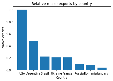
Install nbstripout into the challenge repository. Add the maizeexports.ipynb notebook to the repository and commit it; what messages do you see? Has the notebook been changed in the working directory?

Solution

nbstripout works very quietly—the version of the notebook in your working directory is left unchanged, and no message is given that the committed version has been changed.

Now that the notebook is version controlled, do some tidying of the repository:

• Adjust the notebook to output to files rather than the screen
• Attribute authorship for code that you didn’t write
• Add documentation of what the notebook does
• Adjust the run instructions to include the new tool

Key Points

• Jupyter Notebook can be run in a non-linear order, and store their output as well as their input

• Remove all output from notebooks before committing to a pure code repository.

• Test notebooks from a fresh kernel, or run them from the command line with jupyter nbconvert.

• Use environment variables to pass arguments into a notebook.

Data

Overview

Teaching: 30 min
Exercises: 15 min

Questions

• How do I get data for my code to work on?

• Where should I store data?

• Should data be published?

Objectives

• Be able to pull data from data repositories to operate on.

• Understand options around keeping data with or separate from code.

• Be aware of options around data publication.

As this lesson focuses on code, we haven’t talked a huge amount about data. However, data analysis code can’t do very much without some data to analyse, so in this episode we’ll discuss some of the aspects of open data that overlap with publishing data analysis code. Open data is a huge area, much larger than the scope of this lesson, so we will only touch on some of the outskirts of this; there are many resources available that you can (and should) check out when you get the chance to get a fuller picture.

A first consideration is to decide whether or not the data you are analysing can, or should, be published (by you). For publicly-funded research there is now a general expectation that data should be made public unless there is a compelling reason not to, but there are a variety of reasons that could justify (or even demand) not publishing data. Some examples:

• If the data you are working with is confidential, and you don’t have permission from each person represented in it, then laws in most of the world prevent you from publishing.
• If you have not generated or collected any of your own data, but instead only analysed data from public datasets, then there may be no need to re-publish the data, as it is already available. In this case, a citation is sufficient.
• If you are working with data that is commercially sensitive and have a confidentiality agreement with the company in question, then you may not be able to publish the data, at least without the approval of the commercial partner organisation. Of course, this is likely to also apply to other aspects of your research, even papers or conference talks.
• If your project deals with matters that could affect national security, then there may be even more stringent checks on publishing data or papers.
• If you are part of a collaboration that has not agreed to publish data, then you should not unilaterally publish data, especially if it has been generated collaboratively and not by you personally. You can of course advocate to the collaboration that they should move in this direction. In some cases, collaborations will also have embargo policies that keep data private for a finite period of time to allow collabration members to get as much science as they plan to out of the data, and avoid being “scooped” by another team able to move more rapidly.
• If the data are so large that it is not practical to store or host for extended periods of time, then opening the data may not be possible. This generally only applies to very large experiments or supercomputing facilities, however.

Together or separate?

Assuming that you have decided that your data are publishable, the next question is whether they should be published in the same release as your analysis code, or as a separate package. Once again, there are a number of factors that affect this, but the top two are:

• Is the volume of data significantly larger than the volume of code? If so, then it is likely to be better to keep the two separate, so that those who want to check out and study or re-use your code won’t have to download a large volume of data that they don’t need.
• Is the code likely to be useful in its own right, outside of the specific analysis you have done for the particular publication you’re working on? If so, then again it is likely to be a good idea to keep the code separate, and you may then want to look more closely at packaging your code to make it easier for others to install and run.

If neither of these is true—i.e., the volume of data is pretty small, and the code you have is quite tightly coupled to it, then it may be better to publish the code and data together in a single package. This has the advantage that the two are self-reinforcing; reading the code helps to understand the data, and having the data allows the reader to run the code and see how it works on the data.

Working with open data

As mentioned already, if the data you are working with have already been published, then it is not necessary (or appropriate) to re-publish it. So, what should we do instead?

As in the previous episode about documentation, there are two options: either we describe (in the README or elsewhere) how to get the data to operate on, or we automate the process.

Revisiting our zipf repository, we can see that we have the complete text of two books in our data subdirectory. The books are in the public domain and fully attributed to their authors, and the volume of data is hardly huge, so in principle there is not an urgent reason to omit the data, but conversely its easy availability means that including it isn’t essential either. Let’s see how we could go about removing it.

To create a Git commit that removes files, we can use the git rm command. Similarly to git mv, this combines the rm command with making Git aware of what we have done. Remember that this will only remove the file from the most recent commit; it will still be present in the history for anyone who checks out an earlier commit. (So don’t use this method to remove sensitive data you’ve accidentally committed!)

$ cd ~/Desktop/zipf
$ git rm data/frankenstein.txt data/dracula.txt

Let’s not commit this until we’ve also documented what the user should do instead to get the data that the code expects to operate on. One option would be to place links to the text of the two books in the README, and give instructions to download them and place them in the data directory—after creating it, if we don’t decide to do that.

However, we’ll choose to automate this. To download data from the Internet, we’ll use the curl tool, which is installed as part of most Unix-like systems.

For the time being, let’s recreate the data directory (which Git has helpfully deleted, as there were no files left in it).

$ mkdir data

wget

wget is an alternative to curl that is more specifically designed for downloading files rather than interacting with web servers in general; unfortunately it is not installed by default on some operating systems, so to avoid complexity—both for us and for the users of our published code who would also need to install it—we will stick with curl.

To take a file from the web and place it onto the disk in the file data/frankenstein.txt, we can use the command:

$ curl -L -o data/frankenstein.txt https://www.gutenberg.org/files/84/84-0.txt

The -L flag tells curl to follow any redirects it encounters; the -o tells it to put the data into a specified file on disk (otherwise it would output to standard output). The URL (starting https://…) is something you need to find for your particular data—in this case, it can be found by searching the Project Gutenberg website.

Now that we can download files without needing to click in a web browser, we have all the tools we need to automate getting the data for this paper.

$ nano bin/run_analysis.sh

mkdir -p data
curl -L -o data/frankenstein.txt https://www.gutenberg.org/files/84/84-0.txt
curl -L -o data/dracula.txt https://www.gutenberg.org/files/345/345-0.txt

We should also add a sentence to the README detailing what data the code will work on.

$ nano README.txt

This script will automatically pull the full text of the two books to
process (Frankenstein and Dracula) from Project Gutenberg (gutenberg.org) and place
them into the `data` directory. Internet access is required for this to work.

Now that this is done, we mustn’t forget to commit it back to the Git repository.

$ git add README.txt bin/run_analysis.sh
$ git commit -m 'remove data; retrieve automatically from Gutenberg instead'
$ git push origin main

Getting more data off the web

The procedure above assumes that the data you want to work with is hosted as a simple file that you can download. There is a wealth of data available online in more complex arrangements; for more detail on how this can be accessed programmatically, see the Introduction to the Web and Online APIs.

Dummy data

If commercial, privacy, or other constraints prevent you releasing data for your code to operate on, it is frequently useful to publish dummy data that have the same format as the actual data your code is designed to work with. This will allow readers to check how the program behaves in a trial run, even if the data it returns are meaningless. How to construct dummy data will depend heavily on exactly what kind of analysis you are performing, so we won’t go into more detail about how to create this.

Automated tests

Dummy data is an important part of an automated test system; if you have one, then having the other makes more sense. For more information on automated testing, see for example, Introduction to automated testing and continuous integration in Python

To publish or not to publish

Navia is working on some research that compares two open data sets. She would like to publish her work in an open, reproducible way. In addition to a typical journal output, what else should she publish?

1. Nothing. Her paper should include all the code needed to reproduce the results.
2. A package containing both datasets and the code she used to analyse it. Since the datasets were not originally packaged together and were both used in preparing the work, it is important to include them.
3. A package containing the code for the analysis, and a separate package containing the two datasets used in the analysis.
4. A package containing just the code used for the analysis, which downloads the open datasets.
5. A package containing just the code used for the analysis. The data will be cited in the paper, so is not needed.

Solution

Since the data are already openly available, there is no need for Navia to re-publish them. (Indeed, if she did, it would be misrepresenting others’ work as her own.) The code is likely to be too detailed to be of interest to many readers of the publication, who will instead be interested in the results of the analysis.

So, the answer is either 4 or 5. The exact answer will depend on how the code is written. If it is a general tool for comparing two datasets, then specifying the datasets in the paper may be appropriate. If the code is specific to this publication, then it is more likely to be appropriate to include a tool to fetch the data automatically, since anyone wanting to use the tool will need to use it.

Which of the following should Navia cite in her paper?

1. The datasets used
2. The publications where the datasets were first presented
3. Whatever is specified in the CITATION file for the datasets
4. Any repositories where Navia has published code or data that were used for this paper.
5. Any repositories where Navia has published code or data, regardless of whether they were used for this paper.

Solution

1. Yes, these definitely need to be cited
2. If the original publications helps to understand the provenance or context of the data, or is necessary to support the narrative of this paper, then yes this could be cited. Otherwise, it would depend on the CITATION file of the dataset.
3. Yes, it is usually a good idea to cite work in the form requested by the originators of the data.
4. Yes, publishing your code but not citing it makes it hard to find, so many readers may not realise it is available. Adding a citation in the paper flags the existence of the published analysis code, so that the interested reader can see it, while others do not need to dwell on it.
5. No, only tooling that is specifically relevant to the work in this paper should be cited.

Get some data

Use curl to download the Pakistan biomass field survey from the World Bank. This file is currently included in the repository as surveys.csv. Adjust the script in the challenge repository so that this is downloaded automatically as part of the analysis.

Since this file is now obtained automatically, there is no need to keep the copy in the repository. Remove it, and commit and push these changes.

Key Points

• Use curl to download data automatically.

• For small amounts of data, and code that is specifically to analyse only those data, data and code can be stored and published together.

• For large datasets, or where code is used for multiple different datasets, keep the two separate.

• Data can be frequently be published, if there are no constraints preventing it. If data are not published, then publishing analysis code becomes less valuable.

Reproducible software environments

Overview

Teaching: 20 min
Exercises: 20 min

Questions

• Why do I need to document the software environment?

• How do I document what packages and versions are needed to reproduce my work?

Objectives

• Understand the difficulties of reproducing an undocumented environment.

• Be able to create a requirements.txt and environment.yml file.

So far, we have focused on getting the code that we have written in to a form where another researcher can run it in the same way. Unfortunately, this isn’t enough to ensure that the analysis we have done is reproducible. Each of the libraries we rely on in our code is constantly being developed and updated, as is the Python language, and the operating system that it runs on. As this happens, the default version to be installed on request will change. While minor version changes typically do not introduce any incompatibilities, eventually almost all software needs to introduce changes that break backwards compatibility in some way in order to develop and improve functionality available to new code. In the best case this will cause cosmetic changes, and the next best the code will fail to work at all because some function has been renamed, relocated, or removed. The worst case is when the code still runs without error, but gives a very different answer to that obtained with the old version of the library.

To make our analysis fully reproducible, we need to reproduce the entire computational environment that was used to perform it. In principle, this includes not only the version of Python and the packages that were installed, but also the operating system and the underlying hardware! For now, we will focus on reproducing as much of the original environment as we can.

Exporting environments with Conda

The Conda package manager used by Anaconda gives a way of exporting the current environment. This includes more than just Python packages; it also includes the specific Python version, as well as some dependency packages that would otherwise need to be installed separately. We can export our Conda environment as:

$ conda env export -f environment.yml
$ cat environment.yml

By convention the filename for conda environments is environment.yml; this file is in YAML format. Looking at it, we see it encodes the environment name, the Conda and Pip packages that we have installed, as well as the path to the environment on our computer.

If you don’t use Conda

We have used Conda here because it can define things quite precisely, including the version of Python and many external dependencies in addition to the Python packages being used. However, if you don’t use Conda, you can still export an environment.

The most basic way is built into Pip. Using pip freeze will output a list of all currently installed Pip packages. While this will not work if you are using Conda, since these packages are not available through PyPI, if all your packages were instead installed through Pip, then this gives a very commonly-accepted way to document your environment. By convention the filename for your list of packages is requirements.txt.

$ pip freeze > requirements.txt

Another alternative tool is called Poetry. This combines some of the functionality of pip freeze with some of the dependency and environment management aspects of Conda.

Trimming down an environment

We can see that this file is rather long; this is because we have exported the Anaconda base environment. This comes with a huge array of packages that could be useful for doing scientific computation. However, it means that it will be a lot of data to download for anyone who wants to recreate the environment, and a lot of that data will not be needed as it is packages we haven’t used. Instead, let’s create a new, clean environment to export, starting from Python 3.9

$ conda create -n zipf python=3.9
$ conda activate zipf

Now, we can install into this environment only the packages that we refer to in our Zipf code. If we haven’t documented all the requirements in the README yet, we can work out what these are by looking for any import statements in our code, and identifying those that are not either provided by our own code or by the Python standard library.

$ grep -r --no-filename import bin | sort | uniq

from collections import Counter
import argparse
import csv
import matplotlib.pyplot as plt
import pandas as pd
import string
import sys
import utilities as util

Of these, collections, argparse, csv, string, and sys are all part of the Python standard library, and utilities is part of our own code. That leaves Matplotlib and Pandas. Let’s install these with Conda:

$ conda install pandas matplotlib

If we’re using any tools installed without importing them, then they won’t be picked up by grep; in that case we need to check through our shell scripts to see if any commands are being run that need to be installed. If your analysis includes Jupyter Notebooks, for example, then you will need jupyter installed, even if you don’t ever use import jupyter.

Conda can also provide tools that aren’t Python packages, like curl. If you’re using a tool, or a specific version of a tool, that is likely to not be installed on everyone’s computer, then you should specify that too. curl is installed on most operating systems as of 2023, but it is possible that somsone will need it.

$ conda install curl

It’s a good idea to do a quick check now that this environment can indeed run our analysis, in case we’ve forgotten anything:

$ bash ./bin/run_analysis.sh

Let’s export the environment again in both formats:

$ conda env export -f environment.yml
$ cat environment.yml

These files are now much shorter, so will be much quicker to install.

Spot the difference

Take a look at the following plot of cattle populations by country, which was generated by a Python program using Matplotlib on an older computer.

Try and run the cattlepopulations.py file yourself. Does the output you see look the same as the one above? If not, why not?

Solution

Matplotlib changed its default style set with version 2.0, so the colours of plots made with the default styles changes between the old and new versions. Also, the default behaviour of bar charts is to centre the labels, where to achieve this before you needed to do extra work.

This is why we must specify our environment when we share our code—otherwise, other people will get different results to us. In this case it was just the formatting of a plot, but in some cases it will be the actual numerical results that will differ!

As an aside, in fact there have been other changes to bar charts so that they are easier to make. Specifically, the positions variable is no longer necessary at all, you can use:

plt.bar(countries, cattle_numbers)

and achieve the same results as the file above did.

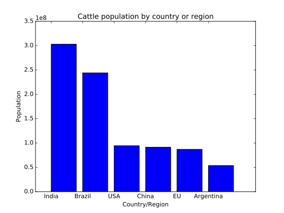
Containers

A popular, but somewhat more involved, alternative to using these kinds of environment is to use containerisation, with products such as Docker and Apptainer (previously Singularity). This is beyond the scope of what we’re covering in this lesson, but the Carpentries Incubator provides an excellent lesson on getting started with Docker that is worth looking at if you are interested.

Define another environment

Create a new Conda environment with just the packages you need for the challenge repository, and export an environment.yml file. How long is this file compared to the one for the base Anaconda environment?

Solution

Since this analysis includes running a Jupyter notebook, we need to have Jupyter installed in addition to the packages that are imported in our code.

$ conda create -n challenge
$ conda activate challenge
$ conda install numpy matplotlib pandas jupyter
$ conda env export -f environment.yml

The environment for the challenge repository’s requirements should have around 125 lines, while the full Anaconda environment is over 300 lines.

Using pip and requirements.txt

Try and create an environment for the challenge repository that installs packages via pip and export it to a requirements.txt file.

Solution

Firstly, create a new Conda environment with just Python.

$ conda create -n challenge_pip python=3.9
$ conda activate challenge_pip

Now, install Python packages only using pip, not with conda.

$ pip install numpy matplotlib pandas jupyter

~~ {: .language-bash}

If your project depended on non-Python packages (for example, recent versions of CMake or GNU Make), then you could still install these from Conda.

Now, to export a requirements file:

$ pip freeze > requirements.txt

We could still use conda env export here to generate an environment.yml file, and it would list our packages installed from pip, under a specific entry designating that they were installed via pip.

Key Points

• Different versions of packages can give different numerical results. Documenting the environment ensures others can get the same results from your work as you do.

• pip freeze and conda env export give plain text files defining the packages installed in an environment, and that can be used to recreate it.

Verifying your analysis

Overview

Teaching: 20 min
Exercises: 20 min

Questions

• How can I use environment definitions to get started on a new machine?

• How can I check that my analysis is working?

• How do I verify that the environment definition is correct?

Objectives

• Be able to use pip and conda to create new environments from definition files.

• Be able to test that an analysis gives correct result.

• Be able to use MyBinder to test code in a clean environment.

Creating an environment from a definition

Having exported our environment, it would be useful to check the reverse process. How do we turn an environment definition into an environment we can use? Conda gives us the tools to do this, too.

$ conda env create -f environment.yml -n conda-test
$ conda activate conda-test

Then, we can re-check that the created environment runs the analysis just as well as the original:

$ bash ./bin/run_analysis.sh

Now that we’ve tested that it works, we should add the environment to our repository.

$ git add environment.yml
$ git commit -m 'define software environment'
$ git push origin main

What about requirements.txt?

If you have a requirements.txt instead of an environment.yml, then you can install the required packages with Pip using

$ pip install -r requirements.txt

This will work inside a Conda environment, but Conda is not required—any number of solutions (e.g. venv, pipenv) could be used instead.

Running on someone else’s computer

We’ve now verified that we can recreate the computational environment we used for a piece of work. However, we have only done this on our own computer. Since other researchers won’t have access to our computer, it would be good if we could test on neutral ground, to check that the analysis isn’t specific to our own machine, but will run elsewhere as well. Even better would be if we could also run any researcher’s (public) code there, to avoid needing to download each and fill our disk with Conda environments as we explore what open software is available.

There is a tool that will help with this called Binder. This is a piece of software that will identify the environment requirements (looking for files like requirements.txt and environment.yml) and automatically build a “container” that runs exactly the software requested. No matter where in the world you are, it will end up with the same operating system and package versions. Once it has built the environment, it will then launch a Jupyter Notebook environment for you to run the code from the repository. The primary design of Binder is to enable exploring others’ data, but it also works for testing environments and running code outside of notebooks.

There is a public Binder instance available at MyBinder, which we can use for testing. (This is run on a relatively small budget, so sometimes it is short on resources; you shouldn’t treat it as a free resource to run long-running computations on! If you need to run Binders regularly, or need compute resources bigger than what you have on your own machine, then talk to the research computing group at your institution, who are likely to have suggestions on where to turn.)

To test our zipf repository and its environment, we can enter the URL to the repository into the MyBinder home page. In principle we could test the repository state at any point in its history, and launch a specific notebook if we wanted. For now, we will test the most recent commit, and launch the Binder without targeting any one notebook. The environment takes a while to build, as it has a number of setup steps. (Unfortunately, the MyBinder service has limited resources, so sometimes will fail to build or fail to load due to lack of capacity or other maintenance issues.)

If you want to encourage others to explore your data with Binder, the home page also gives you the option to add a badge to your README that will take users directly to a new Binder for the repository without needing to type the details in by hand.

Testing, testing

Create a clean Conda environment on your computer based on the specification, in the challenge repository, and use it to re-run the analysis. Does it work, and give the same results as when running it in the environment you were previously using?

If not, try to work out (or ask a helper) why the results are different.

Another Binder

Start a MyBinder instance for your challenge repository. Try running the full workflow on MyBinder. Does it gives the same results as you see running on your own machine?

If not, try to work out (or ask a helper) why the results are different.

Key Points

• Use pip install -r and conda env create to create a new environment from a definition.

• Running your full analysis end-to-end in a clean environment will highlight most problems.

• Binder services (e.g. MyBinder) will create an environment in the cloud based on your definiiton.

Publishing in open science repositories

Overview

Teaching: 20 min
Exercises: 20 min

Questions

• How is an open science repository different to something like GitHub?

• How do I create a permanent version of record of my code?

• How can I create a DOI for my code and cite it?

Objectives

• Understand the difference between the various types of repository.

• Understand how to push a repository from GitHub to Zenodo.

• Be able to find the DOI for a repository and cite it.

So far we have been working to tidy our repository and make it reproducible, pushing and pulling work to and from GitHub. However, at the end of any drafting process there comes a point where you declare the work finished, and make it available as a finalised version of record—for a paper this is where you submit to a journal and (hopefully) have the paper published. Similarly, we would like to make a finalised version of our code available, to give an indication that:

• The code is finalised, and the version presented is the version used to perform the analysis for any publications based on the code. By analogy, we wouldn’t link colleagues to the online collaborative editable version of our paper instead of publishing in a journal.
• The code will be available for the long term. While GitHub has been around for a while, it makes no promises as to long-term availability. Published academic journals are available from decades or centuries ago; drafts and collaborative notes from that period are harder to find.
• We would like the code to be treated (and cited) as an academic output. GitHub is popular with and well-known among software engineers, but in academic circles it is less familiar, or at least is known as a website to get free software from; the idea of software (code) being valuable in and of itself is more novel. Having a repository similar to the more familiar preprint repositories, and that can assign a DOI to a peice of work, will hopefully better align your work as an object worthy of academic consideration.

DOI?

DOI, short for Digital Object Identifier, is a type of unique identifier most frequently used to identify academic journal articles, but which can also be used for other “digital objects”, including data sets as well as, for example, official publications of the European Union. It is designed to be more permanent than a URL, since internet locations may change over time as journals or their publishers change names. They can look like doi:NNNN.MM/XXX where NNNN, MM, and XXX are numbers; they can also be formatted as https://doi.org/NNNN.MM/XXX. The latter can be entered into a browser, and doi.org will always redirect to the current location of the object.

Publish in a data repository

One good option for publishing code is to use a data repository. There is a wide range of data repositories available, many of which are specialist towards particular disciplines. Many potential venues for publishing software (and many other digital services to enable open science) can be searched at the European Open Science Cloud. It’s also possible that your institution hosts its own data repository, and/or mandates a specific one. Your institution’s Open Research or Open Data policy, if it has one, should have more detail on this.

Today we’ll look at a general-purpose data repository called Zenodo. Zenodo is hosted by CERN (the European Centre for Nuclear Research in Geneva), and is part of the same infrastructure that manages the collossal amounts of data generated by the Large Hadron Collider. The computing resources supporting it have operational plans and budgets reaching decades into the future, which is about as long-term as any services currently operate on.

Keep your tests separate from your real data

Because Zenodo is designed to keep research data safe for the long term, it’s not a good idea to upload test or toy data to it. For that reason, for this lesson we’ll be using the “sandbox” version of Zenodo. This behaves exactly like the real version, but is regularly purged of new datasets, and isn’t where you should publish your actual research outputs! Remember to go to the real Zenodo once you’re ready to publish your research.

To publish on Zenodo (and Zenodo Sandbox), we first need to create an account.

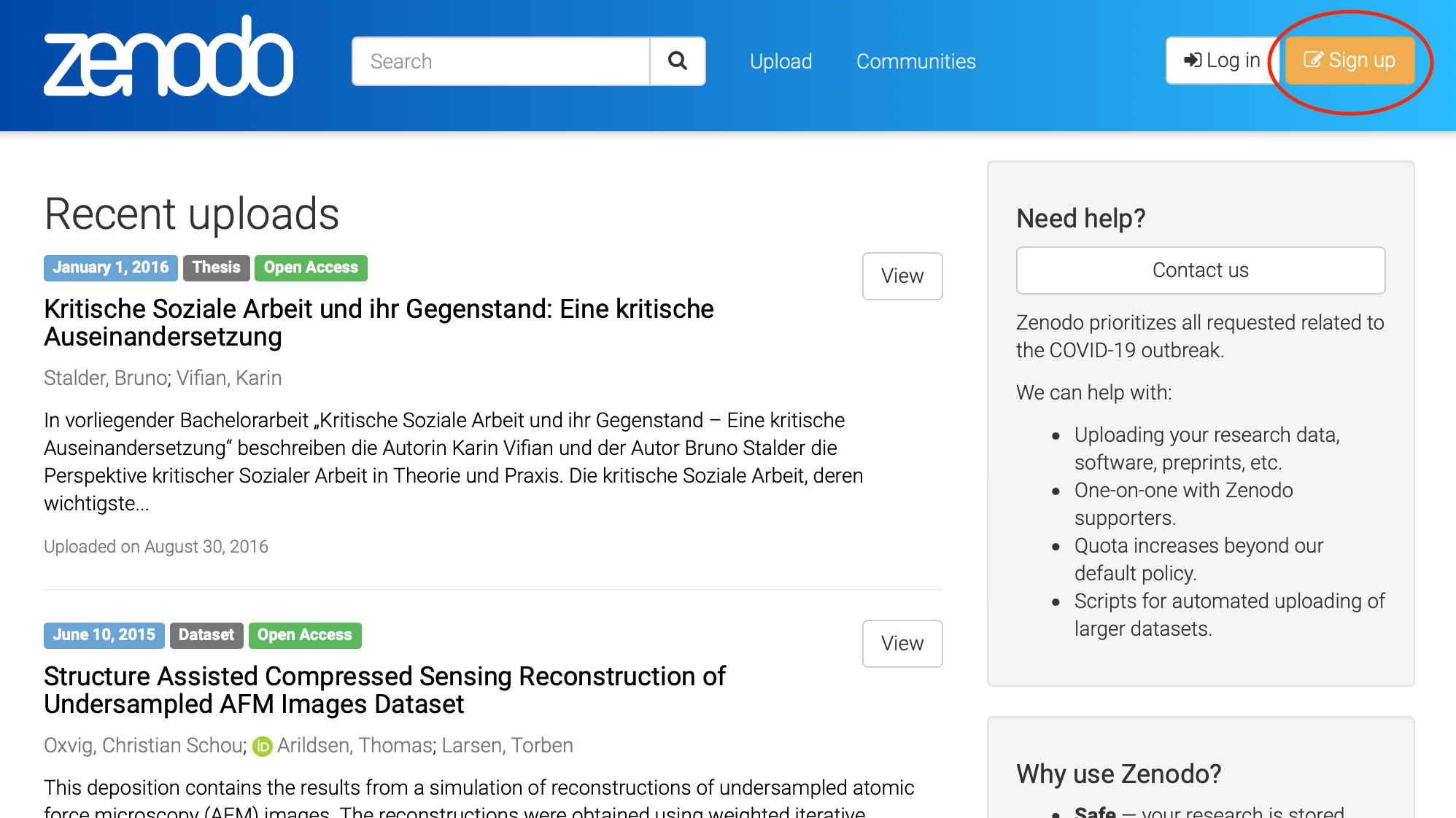
While this can be done manually, the quickest way for our purposes is to log in using GitHub. This will connect our GitHub account with our Zenodo account. If you have one, you can also link your ORCID to your Zenodo account, so that your publications on Zenodo are easier to tie back to your work in other venues.

Once we are signed up and logged into Zenodo (Sandbox), we can use the drop-down next to our email address at the top-right to select the GitHub option.

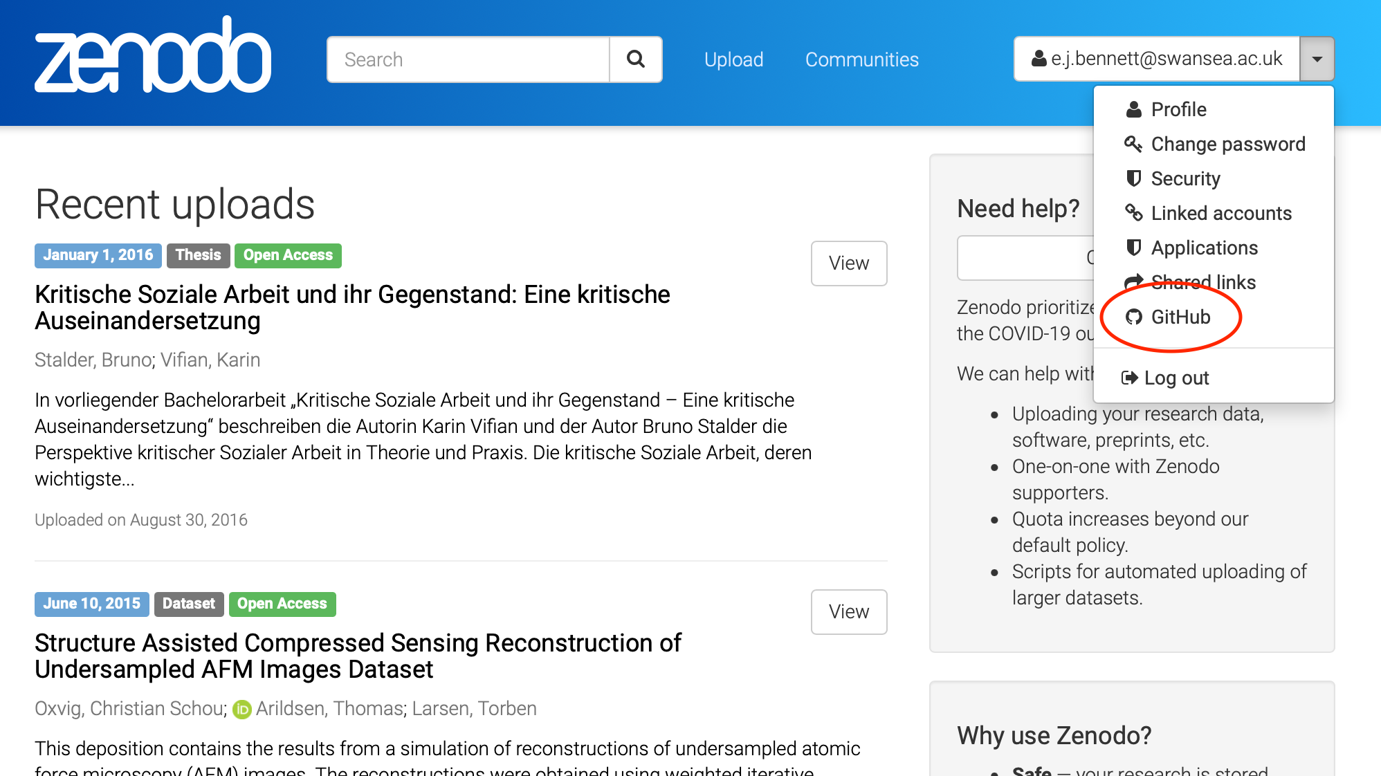
This gives us a three-step process to publish our repository to Zenodo. Firstly, out of the list of repositories presented (found from our GitHub account), we choose which we want to publish to Zenodo. Let’s do that now for the zipf repository.

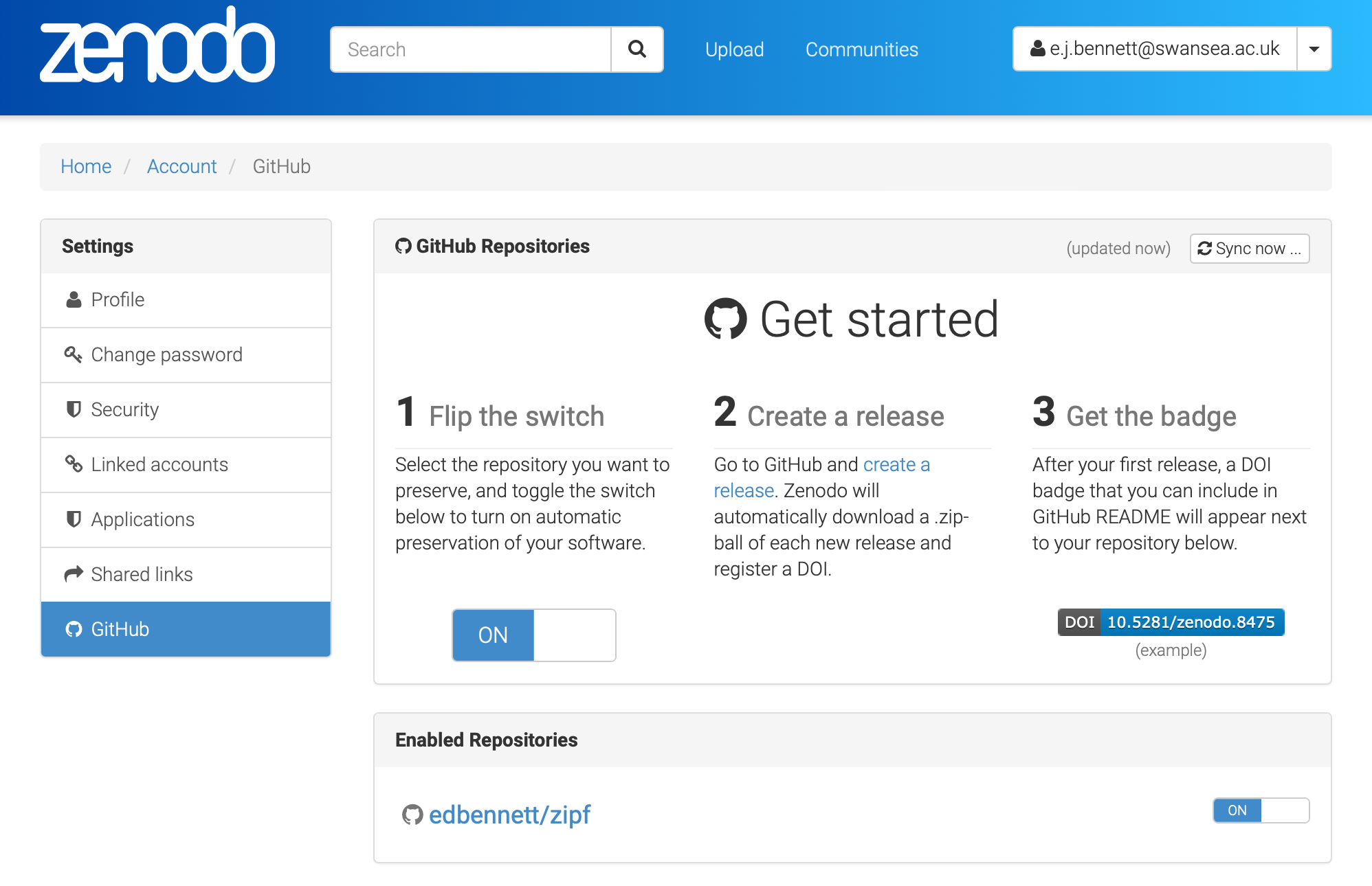
Once this is done, we need to create a “release” of our code on GitHub.

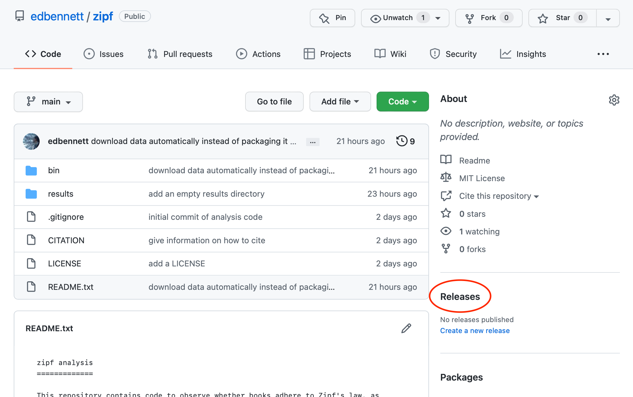
To do this, we can click through from the repository home page to the Releases page, and from there click the “Create a new release” button.

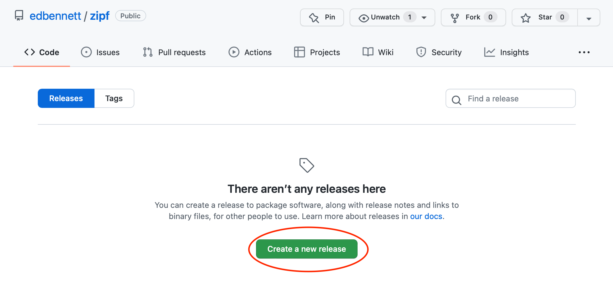
The form to create a new release requests some information

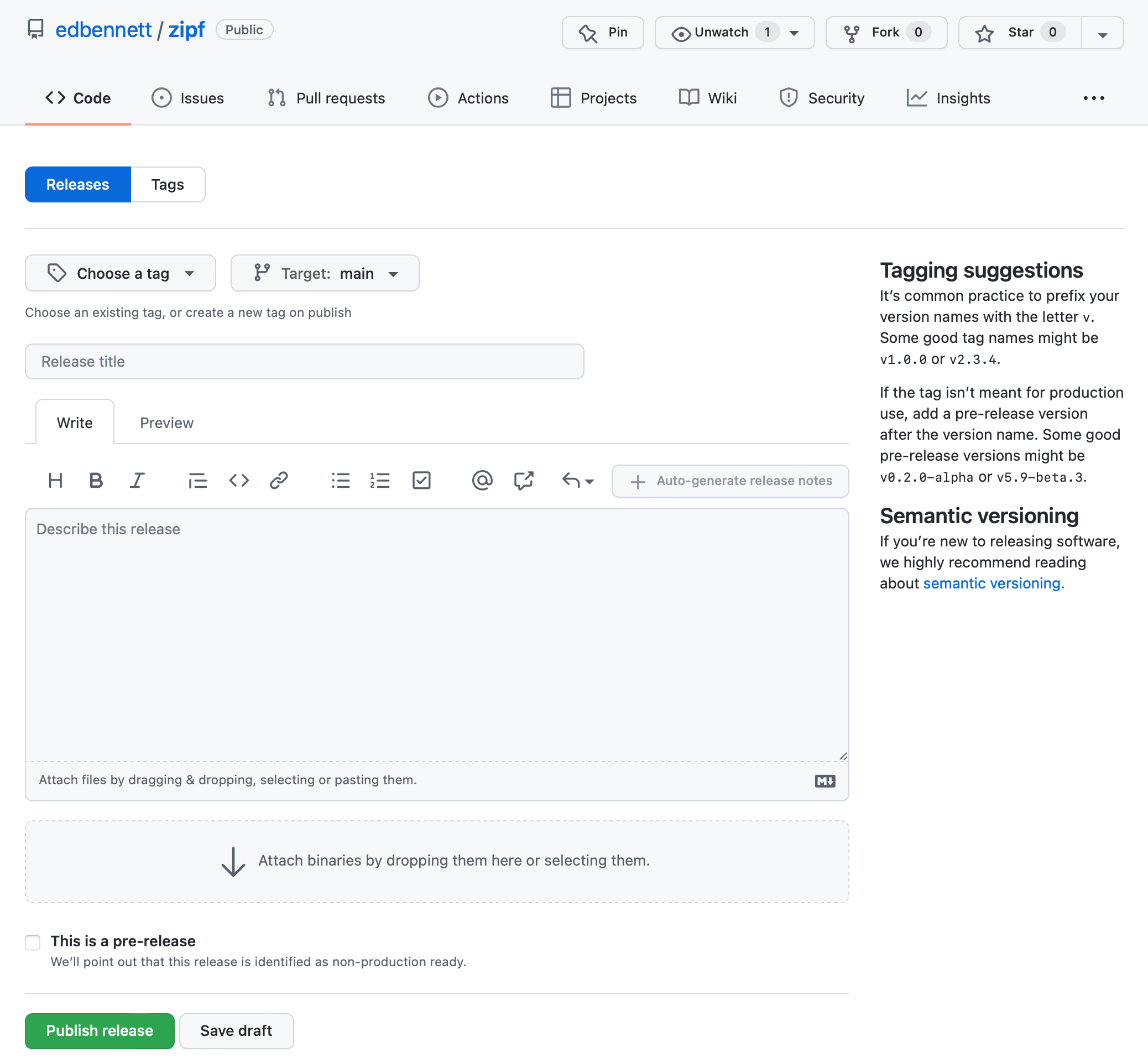
• Choose a tag: If you use tags in your repository, you can choose which tagged commit should be released. If not, then GitHub can automatically create a tag for you when you publish the release—type the name you want the tag to have in this box. This will frequently be the same as the release name.
• Target: this should be the branch that you are releasing from. This will most likely be the main branch.
• Release title: This should be a version name for the particular release. This is designed for software that gets regular releases, or at least more than one in its lifetime. For a piece of data analysis code that is specific to one publication, it is enough to use v1.0.0 here.
• Describe the release: Some more discussion of the release can in principle go here. Note that this is describing the release, not the code—the code (and underlying research) should be discussed in the README. This is again more useful when you are releasing multiple times; each release should use the description to outline the changes included since the previous release.
• Attach binaries: We can ignore this; if we were publishing software written in a language like C or Fortran, and that we wanted others to be able to install, we could attach the compiled versions of the program here.

Once we have filled out the form, we can click Publish, and Zenodo (or the Sandbox) will pick up that we have created a release, and will create a corresponding data publication. It will also then create a DOI, which you can add to the bibliography of any papers that use results generated by the code. This will take a while (a few minutes to an hour); you can check the status by clicking on the repository in the listing on Zenodo.

The third step suggested by Zenodo is to add a badge to our README. Since we have used plain text for our README, that will not work, but if you were using Markdown, you could copy and paste the code generated by Zenodo to add the DOI of the repository, so that readers arriving to the GitHub repository page are aware that they can cite the code via DOI as well.

Alternatives publishing routes

For tools that can be applied more broadly, there are some alternative routes to publication (that can be used instead of or in addition to Zenodo).

1. Publish a package. Depending on the venue, this may or may not aid citability. For example, publishing a Pip package will not enable citation, but publishing to WorkflowHub publicly will create a DOI.
2. Publish a paper. There are publications that specifically enable promotion and constructive peer review of research software. The Journal of Open Source Software connects to GitHub similarly to Zenodo, but requires a very short “paper” explaining the context of what the software does. This allows you to get some feedback from other computational researchers on your code.

Home turf

Try and find your own institution’s policy on open research or open data. Does it have a local repository for source code (or research data more generally), or recommendations on where to publish it?

Fitting in

Are there any discipline-specific repositories for data or code that are in use in your discipline?

Discuss with a neighbour, or in breakout rooms.

Versioning

Wei published the analysis code for his last publication about bat biomechanics on Zenodo. Now he has prepared a new paper about squirrel biomechanics, making use of a lot of the same code, but with some modifications to make it applicable to squirrels rather than bats. He is wondering how best to publish this modified code. What would be the best option for Wei?

1. Publish the new version of the code entirely separately, with a citation to the bat code.
2. Publish the new version of the code entirely separately, with no mention of the bat code.
3. Create a new version of the previous published code on Zenodo, and update the metadata to indicate that the code is now squirrel-specific.
4. Keep the updated code on GitHub, but keep citing the DOI for the bat version of the code, since it links back to GitHub where the updated code is.
5. Something else?

Publish the challenge

Enable preservation of the challenge repository in the Zenodo Sandbox. Create a new release, and get the DOI from Zenodo.

What next?

In this lesson we have focused primarily on taking a piece of code that has already been written and adjusting it to prepare it for publication. Of course, as you do this, your habits in writing software will change so that for future publications the workload is less—perhaps you keep things in Git from the start, choose a directory structure, and write a README as you progress through your work. As you gain experience, the process of publishing your analysis code will become second-nature.

If you do continue down this road, you might find it useful to have tools that nudge you towards a neater structure from the moment you start your project. One such tool that is also popular with professional software engineers is called Cookiecutter; this gives you access to a variety of project templates that are appropriate for particular types of project. In particular, there is a Cookiecutter template for data science that will give you a project structure similar to the one we have discussed in this lesson (along with some other suggestions that we haven’t had time to cover).

Key Points

• Source code hosts like GitHub are designed for active development of software. Open science repositories are to keep versions of record for the longer term.

• Services like Zenodo allow you to package a particular commit, archive it, and give it a permanent identifier.

• Many services like Zenodo will automatically give you a DOI for any dataset, including repositories pulled from GitHub.

• DOIs for code repositories can be cited in journal articles the same way as any other publication.